Reranking with Cross-Encoders: the step that separates good search from excellent search

This post closes out a series. The first one covered semantic search, the second covered hybrid search with Reciprocal Rank Fusion. If you landed here cold: BM25 nails the literal and misses the meaning, vector search does the opposite, and RRF merges the two rankings using position alone, with no weights to calibrate.
Post 2 ended on an open problem. The query in that article was running shoes for hot weather, and the dry-fit tee finished in second place after fusion. It wasn’t what the user wanted, but both retrievers found it plausible, and RRF ranks by consensus of position. Consensus isn’t relevance.
The underlying reason is that up to this point in the pipeline, nobody has read the query and the document together.
What a bi-encoder never actually does
The mechanism is worth being precise about, because the difference between the two setups is the whole story.
In vector search, the embedding model processes the document on its own, at index time, and emits a vector. Months later a query shows up, the model processes the query on its own, emits another vector, and the system compares the two with cosine. That arrangement has a name: bi-encoder. Two independent encodes, and one late, cheap meeting between two points in space.
That’s what makes vector search viable at all. The heavy work happens offline, once per document, and all that’s left on the request path is a geometric comparison. It’s also what makes HNSW possible: you can only build a neighborhood index if the document vector exists before the query arrives.
And that’s precisely where the ceiling is. The vector for “Dry-fit tee for running in the heat” was computed without anyone knowing the question would be about shoes. It has to represent the entire document, for every conceivable query, in 1024 fixed numbers. It’s lossy compression, and what gets lost is exactly the interaction: which parts of this document matter for this question.
A cross-encoder tears that arrangement down. It takes the (query, document) pair concatenated into a single sequence and runs one forward pass over both at once. Every query token can attend to every document token, and the other way around, across all layers. The output isn’t a vector, it’s a number: how well this document answers this query.
The original implementation, from Nogueira and Cho’s 2019 paper, is almost embarrassingly plain. The query goes in as sentence A, the passage as sentence B, the [CLS] token vector feeds a single dense layer, and out comes the probability that the passage is relevant. The query gets truncated to 64 tokens, the whole thing to 512. No new architecture. Just BERT reading both things at the same time.
How big the gain actually is
That same paper has the number that, in my opinion, is the strongest argument for reranking, and it’s strong because it isolates the variable.
On MS MARCO, the candidate set was held fixed: BM25’s top 1000 for each query. BM25 on its own, ranking those same thousand documents, gets MRR@10 of 16.7 on the dev set. A BERT Large reordering the exact same list gets 36.5.
No new documents entered. No index changed. No embeddings were generated. Retrieval was identical in both cases, and the metric more than doubled purely because something read the pairs.
Worth noting what that number doesn’t say. It’s a 2019 benchmark, in English, on a dataset of Bing questions with roughly one relevant passage per query. Your domain isn’t that. But the asymmetry it exposes between “retrieving” and “ordering” is structural, and it shows up again in every benchmark since. Elastic, measuring their own model across 21 BEIR datasets, reports an average 40% improvement in ranking quality when reranking BM25 results.
Why you can’t just run this on everything
If cross-encoders are that much better, the obvious question is why not throw out the index entirely and score every document directly.
The answer lives in the word “pair”. A bi-encoder does N document encodes once in its life, then one encode per query. A cross-encoder does one forward pass per (query, document) pair, every single time, because the score depends on both. There’s nothing to precompute. Change the query and all prior work is garbage.
You can put numbers on this using the published sentence-transformers table, which measures throughput for the MS MARCO cross-encoders on a V100 GPU:
| Model | nDCG@10 (TREC DL 19) | MRR@10 (MS MARCO Dev) | Docs/sec |
|---|---|---|---|
| ms-marco-TinyBERT-L2-v2 | 69.84 | 32.56 | 9000 |
| ms-marco-MiniLM-L4-v2 | 73.04 | 37.70 | 2500 |
| ms-marco-MiniLM-L6-v2 | 74.30 | 39.01 | 1800 |
| ms-marco-MiniLM-L12-v2 | 74.31 | 39.02 | 960 |
| ms-marco-electra-base | 71.99 | 36.41 | 340 |
Take MiniLM-L6-v2, the middle of that list. At 1800 documents per second, scoring 100 candidates costs 56 ms. Scoring a million-document catalog costs nine and a half minutes per query, on a dedicated GPU, for one user. The L12, which buys you half a point of nDCG, takes 17 minutes.
This isn’t something you scale horizontally until it goes away. It’s an order-of-magnitude difference that changes what kind of problem you’re solving.
Look at the third column against the first, too. Between L6 and L12 the quality is essentially identical and the cost doubles. Between TinyBERT-L2 and L6 you buy 4.5 points of nDCG at 5× the time. The diminishing-returns curve is already drawn inside the model family itself, before you’ve even picked a depth.
Hence the architecture everyone converges on: cheap retrieval picks a handful of candidates, and the expensive model only looks at that handful.
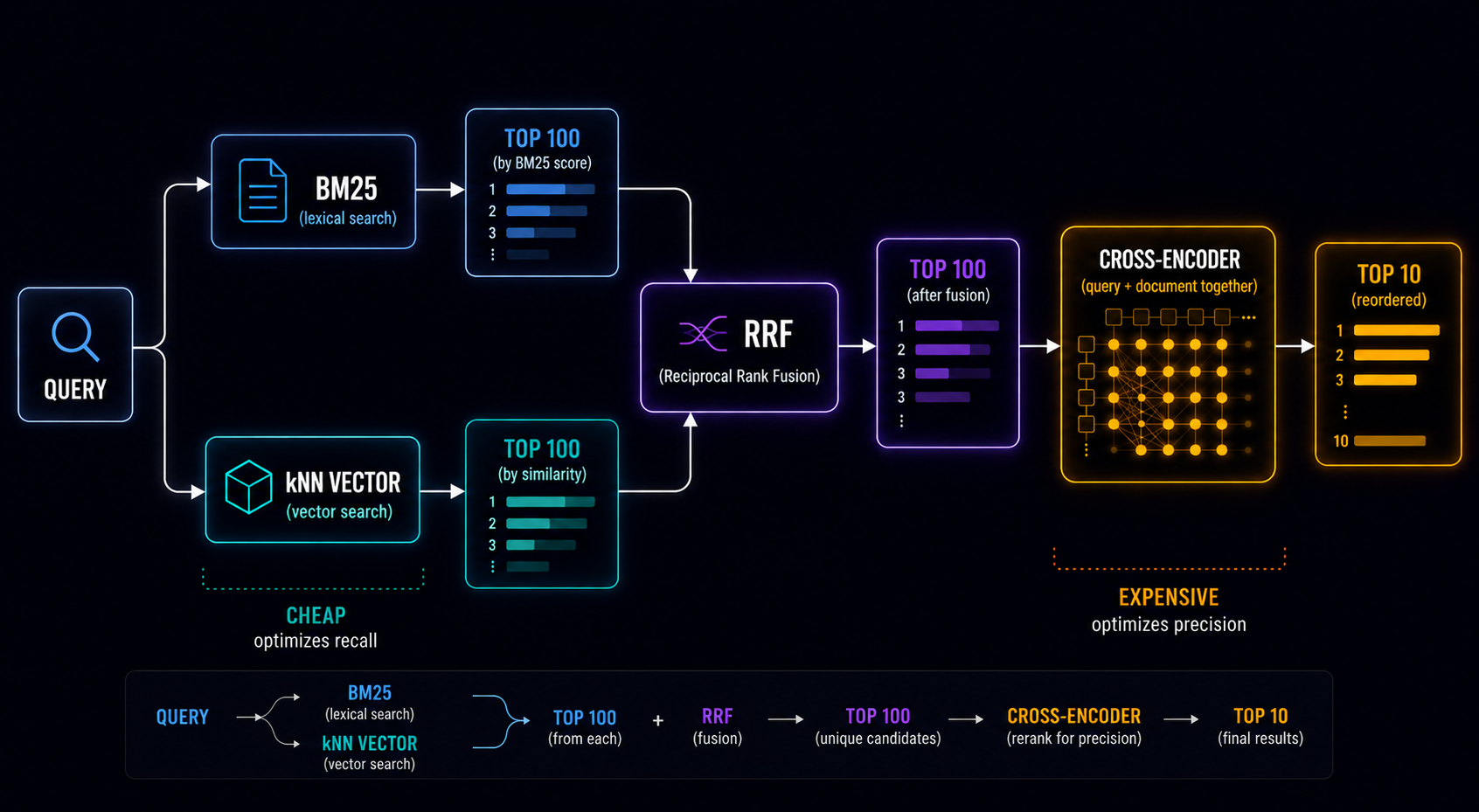
The first stage exists so nothing relevant gets left out. The second exists to get the order right. Different goals, which is exactly why different models make sense.
The tee finally drops
Back to the example from post 2. Five documents, the query running shoes for hot weather, and the ranking RRF produced:
| Position | Document |
|---|---|
| 1 | A: Ventus running shoe, high-ventilation mesh |
| 2 | C: Dry-fit tee for running in the heat |
| 3 | D: Lightweight shoe for hot, humid weather |
| 4 | E: Technical running sock for hot days |
| 5 | B: Rocha 3 trail running shoe, reinforced upper |
Now the cross-encoder gets all five pairs and returns a score for each. The values below are illustrative, but the ordering is what any decent reranker produces here:
| Document | Score | Final position |
|---|---|---|
| A: Ventus, mesh | 0.94 | 1st |
| D: Lightweight, hot weather | 0.91 | 2nd |
| B: Rocha 3 trail | 0.38 | 3rd |
| C: Dry-fit tee | 0.07 | 4th |
| E: Technical sock | 0.04 | 5th |
The tee dropped from second to fourth, and the reason is mundane once you look at the mechanism: the model processed the query token “shoes” in the same forward pass as the document token “tee”. It isn’t comparing two summaries of meaning, it’s reading a question about footwear alongside a document about apparel and concluding the category is wrong, even though “running” and “heat” both match literally.
B climbed to third on the complementary logic. It’s a running shoe, so it hits the primary intent, but “reinforced upper” is the opposite of ventilation, and the model penalizes without discarding. Neither earlier stage can draw that distinction, because neither one read both texts at once.
Notice the gap between 0.91 and 0.38. That isn’t scale noise the way RRF scores are. That’s the model separating two populations.
Picking a model
The ecosystem splits three ways, and the choice is almost never about ranking quality.
Managed API. Cohere Rerank is the reference here. The current line is rerank-v4.0-pro and rerank-v4.0-fast, both multilingual across 100+ languages, with a 32k-token context window and support for semi-structured JSON documents. rerank-v3.5 is still around with 4k. Voyage and Jina play the same game. You add one HTTP call and you’re done: no GPU, no deployment, no reindexing.
The planning detail is the billing unit. A “search unit” is one query with up to 100 documents, and long documents get chunked automatically, with each chunk counting as a separate document. Meaning your 100 candidates can turn into several search units if the texts are large. The AWS Marketplace listing for Rerank v3.5 (Bedrock edition) prices it at $0.002 per search unit. That’s roughly $200 for a month with 100k reranked searches, and $2,000 for a month with a million. Prices change, so check before you commit, but the shape holds: API reranking is cheap per search and expensive per traffic.
Self-hosted open source. The cross-encoder/ms-marco-* family from sentence-transformers is the classic starting point, and the table above already shows the whole trade-off. One warning that matters more than it looks: those models are trained on MS MARCO, which is English. If your corpus is Portuguese, Spanish, or anything else, they will disappoint you. For multilingual work the answer is BAAI/bge-reranker-v2-m3, built on top of bge-m3, with a 512-token window and a score you map to 0…1 with a sigmoid. The BGE docs give the obvious and correct advice: test on your real use case and pick on speed/quality balance, not on their table.
Built into the engine. Elasticsearch exposes reranking through the text_similarity_reranker retriever, which can point at an external inference endpoint (Cohere, for instance) or at Elastic’s own model, Elastic Rerank, a 184M-parameter DeBERTa v3. Read the limitations before you get excited: English only, 512-token window, available from Stack 8.17, requires an appropriate subscription level, and still flagged as technical preview. Elastic writes in their own docs that the preview version may be cost prohibitive for high query rates with low-latency requirements, and recommends staying under top-30 for CPU inference.
The middle option. ColBERT occupies its own niche. Instead of one score per pair, it stores a vector per document token and performs a late interaction between query tokens and document tokens at query time. The original paper measures effectiveness competitive with the BERT models of the day while running two orders of magnitude faster and using four orders of magnitude fewer FLOPs per query. The price is the index: storing a vector per token inflates storage aggressively, and ColBERTv2 exists largely to shrink that by 5 to 8×. If latency is your constraint and you have disk to spare, it’s worth a look.
Depth is the parameter that matters
Here’s the most expensive mistake in this stage, and it runs against intuition.
The default belief is that reranking more candidates can only help, since a good model would have more material to work with. Elastic measured this systematically, sweeping reranking depth across several models and BEIR datasets, and found three patterns:
- Fast rise, then saturation, in 72.6% of cases. What everyone expects.
- Rise to a peak, then decay, in 20.2% of cases.
- Steady decay with any amount of reranking, in 7.1% of cases. The reranker makes BM25 worse at every depth tested. The explanation is mechanical and satisfying. nDCG@10 only moves when the reranker promotes something from below into the top 10. If the promoted document is relevant, the metric goes up. If it’s a false positive, it evicts a relevant document and the metric goes down. As you go deeper, the density of relevant documents collapses and the density of irrelevant ones grows. There’s a depth at which the model’s false-positive rate starts to dominate, and past it you’re paying for inference to degrade your own ranking.
The paper Drowning in Documents gets to the same place from another direction, and notes something uncomfortable: rerankers frequently assign high scores to documents with no lexical or semantic overlap with the query at all.
Three practical consequences, in the order you’ll need them:
First, the number. Applying the rule of picking the depth that reaches 90% of the maximum gain, Elastic landed on roughly top 100 over BM25, at a third of the compute cost of chasing the maximum. When cost is tight they recommend top 30 with their model, and still measured over 40% uplift in nDCG@10 on the QA portion of their benchmark.
Second, which way to tune. The better your first stage, the fewer candidates you need to rerank, because recall saturates earlier. And the better your reranker, the deeper it pays to go, because it makes fewer mistakes on the way down. You already have hybrid search with RRF, so your first stage is good: start shallow.
Third, and this one surprised me: under a latency constraint, reranking deep with a small model tends to beat reranking shallow with a big one. In Elastic’s benchmark, MiniLM-L12-v2 processing 80 candidates beat stronger models capped at 10 or 20 for the same time budget. The relationship flips as you relax the constraint.
On latency, one concrete number to calibrate against: measuring on two T4 GPUs, Elastic reports 0.0869 seconds to score 10 pairs with Elastic Rerank on HotpotQA. Linearized, top-30 lands around 0.26 s and top-100 around 0.87 s. Those aren’t the 50 ms that get thrown around in posts on the topic. Measure on your hardware, with your documents, before you promise an SLA.
Scores mean something again
One limitation I raised in post 2 gets resolved here, and it’s worth closing the loop.
RRF scores mean nothing. They’re crammed into a tiny band, they aren’t comparable across queries, and so you can’t threshold on them. You can’t say “if the best result is bad, show the empty state”.
A cross-encoder score is a different kind of thing. It’s a relevance estimate for that pair, produced by a model trained for exactly that, and it doesn’t depend on anyone’s position. The sentence-transformers models return logits that sit roughly between -10 and 10, and you apply a sigmoid to get something in 0…1. bge-reranker-v2-m3 works the same way. Cohere returns a normalized relevance_score. Elasticsearch exposes min_score right on the retriever precisely so you can cut.
The trap is confusing “meaningful” with “calibrated”. The scale is specific to the model and the domain. A 0.6 from Cohere is not a 0.6 from BGE, and a 0.6 from BGE on your legal corpus is not the same 0.6 on your support FAQ. The threshold has to come from your data. But it exists, and that’s a genuinely new capability in the pipeline.
What this looks like in code
Self-hosted, with sentence-transformers. The point of the snippet is that reranking is a pure function over the candidate list, with no state and no index:
from sentence_transformers import CrossEncoder
import torch

# Sigmoid pins scores to 0..1. Without it you get raw logits.
reranker = CrossEncoder(
    "BAAI/bge-reranker-v2-m3",   # multilingual; for English, ms-marco-MiniLM-L6-v2
    activation_fn=torch.nn.Sigmoid(),
    max_length=512,
)

def rerank(query: str, candidates: list[dict], top_k: int = 10) -> list[dict]:
    """Takes the output of RRF, returns the reordered top_k."""
    if not candidates:
        return []

    pairs = [(query, doc["text"]) for doc in candidates]
    scores = reranker.predict(pairs, batch_size=32)

    for doc, score in zip(candidates, scores):
        doc["rerank_score"] = float(score)

    ranked = sorted(candidates, key=lambda d: d["rerank_score"], reverse=True)
    return ranked[:top_k]
Two decisions are worth a comment. batch_size is what determines whether you saturate the GPU or waste it, and it’s the first knob to turn when latency won’t close. And max_length=512 isn’t cosmetic: anything longer gets truncated, so the model scores the beginning of the text and ignores the rest. If your documents are long, you need to decide deliberately which chunk gets scored instead of letting the tokenizer decide for you.
Same pipeline through an API, with Cohere:
import cohere

co = cohere.ClientV2(api_key="...")

response = co.rerank(
    model="rerank-v4.0-fast",
    query="running shoes for hot weather",
    documents=[doc["text"] for doc in candidates],
    top_n=10,
)

# results carry index (position in the original list) and relevance_score
top10 = [candidates[r.index] for r in response.results]
And inside Elasticsearch, chained onto the RRF retriever from the previous post:
GET /products/_search
{
  "retriever": {
    "text_similarity_reranker": {
      "retriever": {
        "rrf": {
          "retrievers": [
            { "standard": { "query": { "multi_match": {
                "query": "running shoes for hot weather",
                "fields": ["title", "description"]
            }}}},
            { "knn": {
                "field": "embedding",
                "query_vector": [0.21, -0.05, "..."],
                "k": 100,
                "num_candidates": 300
            }}
          ],
          "rank_window_size": 100
        }
      },
      "field": "description",
      "inference_id": "my-reranker",
      "inference_text": "running shoes for hot weather",
      "rank_window_size": 100,
      "min_score": 0.4
    }
  },
  "size": 10
}
Note there are two rank_window_size values in that query and they mean different things. The inner one is how many candidates fusion considers. The outer one is how many of those go to the model. Matching them is the sane default; setting the outer one higher does nothing, because no candidate exists beyond the fusion window.
Where reranking doesn’t help
A few cases where the honest answer is to leave it off.
When first-stage recall is the problem. Reranking retrieves nothing. If the right document isn’t among the 100 that arrived, no model is going to invent it. Before investing in the expensive stage, measure Recall@100 on your hybrid search. If it’s low, the problem is your embedding model, what you indexed, or your fusion window, and reranking will only do a nicer job of ordering a bad set.
When value per search is low and volume is high. The classic long-tail ecommerce situation. Millions of searches, thin margin per transaction, and a relevance gain that may not cover the GPU bill or the API bill. This is a business calculation, not an engineering one.
When the latency SLA is tight. If your p95 budget is 100 ms and search already eats 40, you don’t have room for top-100. You have room for top-20 with a small model, and maybe not even that.
When the query is an identifier. SKU-A4729 doesn’t need semantic understanding, it needs an exact match. Detect the pattern before the pipeline and route around it, same as with hybrid search.
When the corpus is too homogeneous. If your 100 candidates are near-identical to each other, there’s no correct order to discover and the model will just break ties on noise.
What to measure, before and after
You already built the most important piece back in post 2: that set of 50 to 200 real queries with the relevant documents marked by hand. It’s what decides this.
Measure nDCG@10 and MRR for hybrid alone, then hybrid plus reranking, sweeping depth at 10, 20, 30, 50, and 100. What you’re looking for is the shape of the curve, not one number. If it saturates at 30, going to 100 is money on fire. If it drops after 50, you just learned the model doesn’t suit your domain, and you learned it offline, which beats learning it in production.
Alongside that, not afterwards, record the p95 delta and the cost per query. A relevance gain without a latency number next to it isn’t a result, it’s half of one.
Then comes the production A/B, because offline gains from reranking almost always look great and users don’t always notice. The metrics that answer this are CTR on the top positions, query reformulation rate, and conversion. If top-3 CTR goes up and reformulation goes down, reranking is doing real work. If nothing moves, you paid for precision nobody was waiting on.
Closing the series
Five things I wish I’d known before starting on any of this:
BM25 isn’t legacy. It’s the strong baseline you’ll spend the rest of the project trying to beat, and on some tasks you won’t.
Embeddings turn text into geometry, and everything else follows from that change of representation. But the vector is lossy compression, and the losses show up in the most annoying place possible: identifiers, negations, short queries.
RRF is the best return on effort in the whole list. No calibration, no training, consistently better than either side alone.
Reranking is the only stage that reads both texts together, which is why it wins where the others structurally can’t. It’s also the only one that precomputes nothing, which is why it runs over dozens of candidates and never over the catalog.
And the thing that ties it together: none of this gets decided by reading benchmarks. It gets decided with an evaluation set from your own corpus, which takes half a day of tedious work to build and then answers every question that comes after.
This series covered what I wish I’d known before starting with semantic search. If you’re building something similar, tell me what the context is. I’d love to know.
References
- Nogueira, R., Cho, K. Passage Re-ranking with BERT. arXiv:1901.04085, 2019. Paper
- Khattab, O., Zaharia, M. ColBERT: Efficient and Effective Passage Search via Contextualized Late Interaction over BERT. SIGIR 2020. Paper
- Santhanam, K. et al. ColBERTv2: Effective and Efficient Retrieval via Lightweight Late Interaction. arXiv:2112.01488
- Jacob, M. et al. Drowning in Documents: Consequences of Scaling Reranker Inference. arXiv:2411.11767
- Sentence Transformers, Pretrained Cross-Encoder models and Retrieve & Re-Rank
- Elastic, docs for Elastic Rerank and the text_similarity_reranker retriever
- Elastic Search Labs, Exploring depth in a retrieve-and-rerank pipeline
- Cohere, Rerank overview, best practices, and the Rerank 4.0 announcement
- BAAI/bge-reranker-v2-m3 and the BGE Reranker docs
Third and final post in the series on modern search. The earlier ones are Semantic Search and Hybrid Search with RRF.
› Continue reading
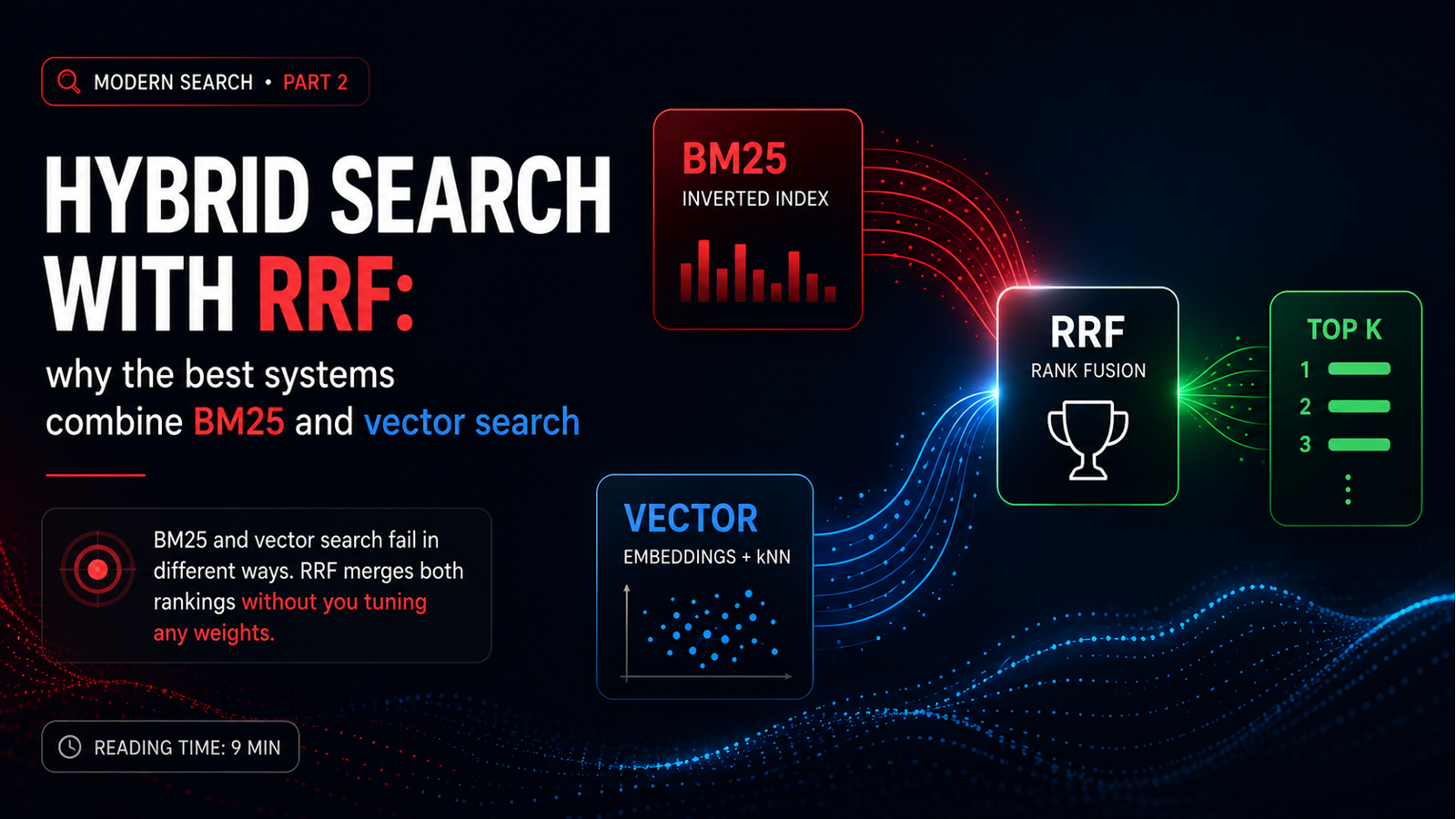
Hybrid Search with RRF: why the best systems combine BM25 and vectors
BM25 and vector search fail in different places. Reciprocal Rank Fusion merges both rankings without you calibrating a single weight. Second post in a series on modern search.
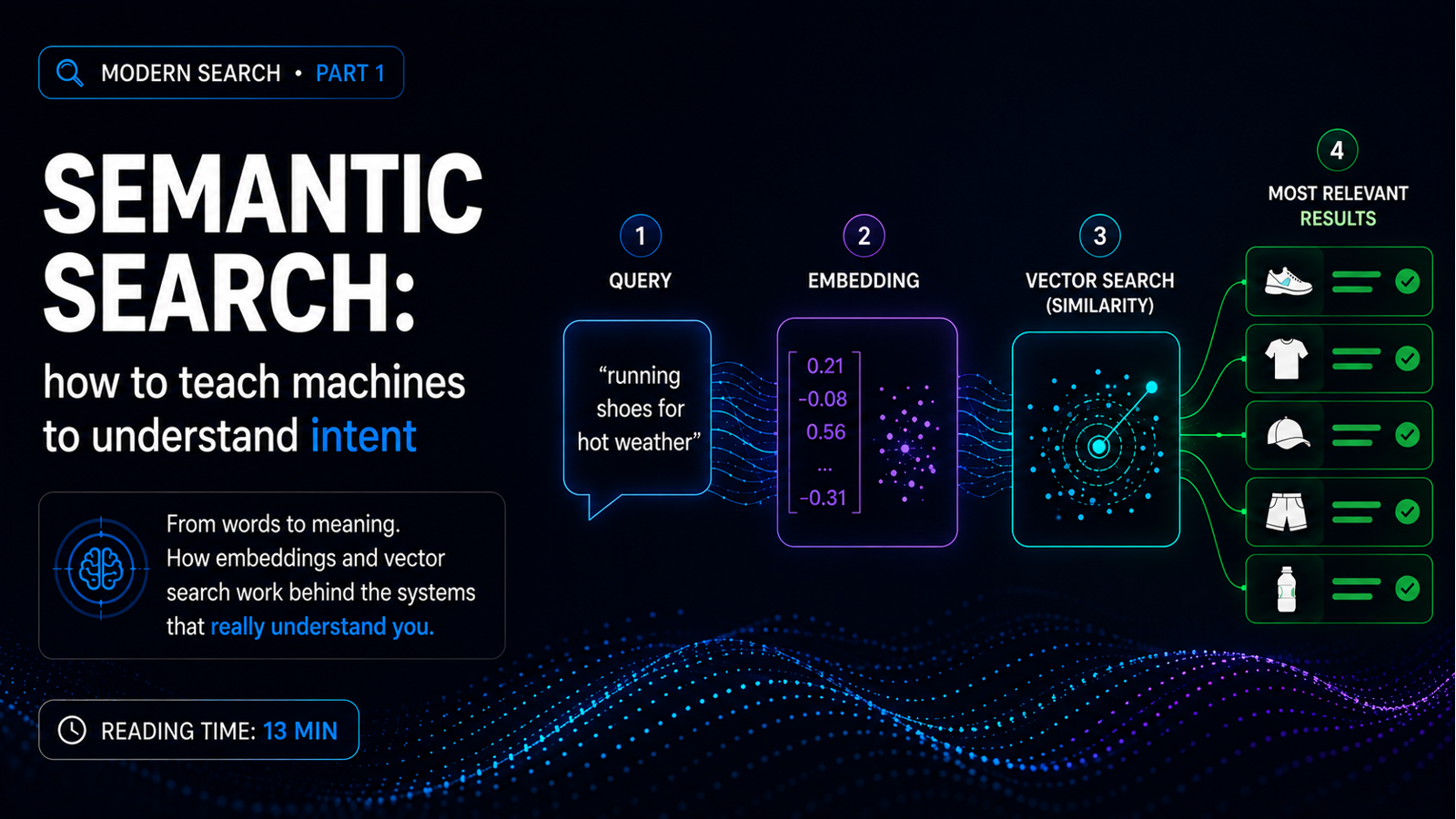
Semantic Search: teaching machines to understand intent, not just words
BM25 still works, but it has four serious blind spots. Embeddings turn text into geometry — and that's the foundation of everything that's hyped in AI today. First in a series on modern search.
Comments
No signup needed. Basic markdown supported. Validated with Cloudflare Turnstile.