Hybrid Search with RRF: why the best systems combine BM25 and vectors
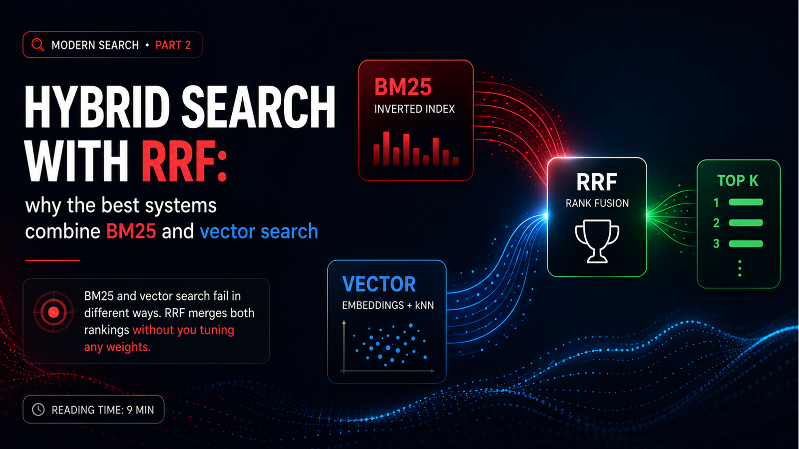
This post assumes you’ve read Semantic Search: teaching machines to understand intent. Two-line recap: BM25 nails the surface of the text and misses the meaning; vector search nails the meaning and misses the literal. The blind spots are complementary, so the obvious move is to use both.
The catch is that “use both” hides a much nastier decision than it sounds.
Two lists on your screen, one results page
Say you’ve run both searches. BM25 returned ten ranked documents. Vector search returned another ten, with some overlap. Now you have to hand the user a single list.
Which document goes in position one?
That’s genuinely the only question hybrid search has to answer. It’s also where most homegrown implementations start falling apart, because the intuitive answer is the wrong one.
Adding the scores looks obvious and almost always breaks
Everyone’s first attempt is a linear combination:
final_score = α × bm25_score + (1 - α) × cosine_score
Neat on paper. Turn the α dial, favor one side or the other, done. Except the two numbers don’t live on the same ruler.
Cosine similarity is bounded: with text, in practice, it sits between 0 and 1. BM25 has no ceiling. Its score depends on term IDF, document length, query length, and corpus size. A single rare term against a million-document index can produce a score dozens of times larger than the maximum possible cosine. Add them raw and BM25 swallows vector search whole. You didn’t configure weights, you configured a scale.
The obvious fix is to normalize first. Per-query min-max, for instance: the best result in each list becomes 1.0, the worst becomes 0.0. And that’s where the trap lives.
Min-max is relative to the query. If vector search found nothing good, the best of the bad results still becomes 1.0. Normalization erased precisely the information that mattered: this list has nothing useful in it. You just handed maximum weight to a terrible result because of an arithmetic rescale.
You can work around it with distribution-based normalization, z-scores, per-domain calibration. All of that works, up to a point. But look at what happened: you showed up to solve ranking and ended up doing score statistics. That α is a hyperparameter that shifts when you swap the embedding model, when the corpus grows, when query mix changes. It’s permanent maintenance.
Rank is universal, score isn’t
Reciprocal Rank Fusion sidesteps all of it by throwing the scores away.
The idea, published by Cormack, Clarke and Büttcher at SIGIR 2009, fits on one line:
RRF(d) = Σ  1 / (k + rank_r(d))
        r∈R
For each ranking r where document d shows up, add the inverse of its position, shifted by a constant k. Sort by the sum. That’s the whole algorithm.
No normalization. No weights to calibrate. No training. Both lists come in as sequences of positions, and a position is a unit every ranker on earth produces identically. BM25’s first place and the vector search’s first place are the same thing: first place. That’s what makes fusion possible without anyone having to answer what a score of 14.7 is worth.
The most important consequence comes for free. Since each list contributes a small, similar increment, the document that rises is the one both searches agree is decent. Not either one’s absolute favorite. RRF rewards consensus.
Five documents, two lists, one winner
Worth watching this happen with actual numbers. Query: running shoes for hot weather, on a sporting goods catalog.
BM25 matches literal tokens and returns:
| Rank | Document |
|---|---|
| 1 | C: Dry-fit tee for running in hot weather |
| 2 | A: Ventus running shoe, high-ventilation mesh |
| 3 | B: Rocha 3 trail running shoe, reinforced upper |
| 4 | E: Technical running sock for warm days |
| 5 | D: Lightweight shoe for humid, warm climates |
The t-shirt takes first place because it matches two discriminative terms, “running” and “hot weather”. It’s useless for the user’s intent, but BM25 has no way to know that. Meanwhile D, which is nearly a perfect paraphrase of the query, sinks: “warm” isn’t “hot” to an inverted index.
Vector search returns a different order:
| Rank | Document |
|---|---|
| 1 | D: Lightweight shoe, warm climate |
| 2 | A: Ventus running shoe, mesh |
| 3 | E: Technical sock for warm days |
| 4 | C: Dry-fit tee |
| 5 | B: Rocha 3 trail shoe |
Now D climbs to the top, as expected. But so does the sock, because “running” and “heat” dominate the query vector and the product category carries less weight than it should.
Each list has a wrong first place, for opposite reasons. Now RRF with k = 60:
| Document | BM25 rank | Vector rank | RRF | Final |
|---|---|---|---|---|
| A: Ventus shoe | 2 | 2 | 1/62 + 1/62 = 0.032258 | 1st |
| C: Dry-fit tee | 1 | 4 | 1/61 + 1/64 = 0.032018 | 2nd |
| D: Lightweight | 5 | 1 | 1/65 + 1/61 = 0.031778 | 3rd |
| E: Running sock | 4 | 3 | 1/64 + 1/63 = 0.031498 | 4th |
| B: Trail shoe | 3 | 5 | 1/63 + 1/65 = 0.031258 | 5th |
A wins without having been anybody’s first choice. It’s the only document both searches put near the top for different reasons: BM25 saw “running” and “shoe”, the embedding model saw “ventilation mesh” and understood heat. That’s consensus doing its job.
Notice what RRF didn’t do: the t-shirt is still second. Rank fusion isn’t a relevance filter. If a wrong document shows up decently in both lists, it stays decent afterward. Hold that thought, it comes back later.
What k actually does
k = 60 gets passed around as a magic number. The origin is far less mystical than that: the paper says the value was fixed during a pilot experiment and never changed in the validation runs that followed.
What the published data does support is the shape of the curve. In Table 1 of the paper, MAP for k between 20 and 100 stays between 0.2134 and 0.2147. Under 1% of variation. The nominal peak is at k = 80, not 60. Only the extremes move the needle: k = 0 drops to 0.2072 and k = 500 to 0.2098.
Translated to your system: k controls how much a single list’s first place counts against consensus.
Take the same shoe example with k = 0, meaning the score is just 1/rank:
| Document | RRF with k = 0 | Final |
|---|---|---|
| C: Dry-fit tee | 1/1 + 1/4 = 1.25 | 1st |
| D: Lightweight | 1/5 + 1/1 = 1.20 | 2nd |
| A: Ventus shoe | 1/2 + 1/2 = 1.00 | 3rd |
The order flipped. With a small k, the gap between first and second place is huge, so each ranker essentially drags its own favorite onto the podium and consensus loses. With a large k, positions become nearly indistinguishable and what’s left is vote counting.
k = 60 is a reasonable balance point on that spectrum, not a global optimum for your domain. If you have an evaluation set, sweep the range. If you don’t, tweaking k by intuition is the last thing that’ll improve your results.
What this looks like in the architecture
The flow is simpler than most people expect:
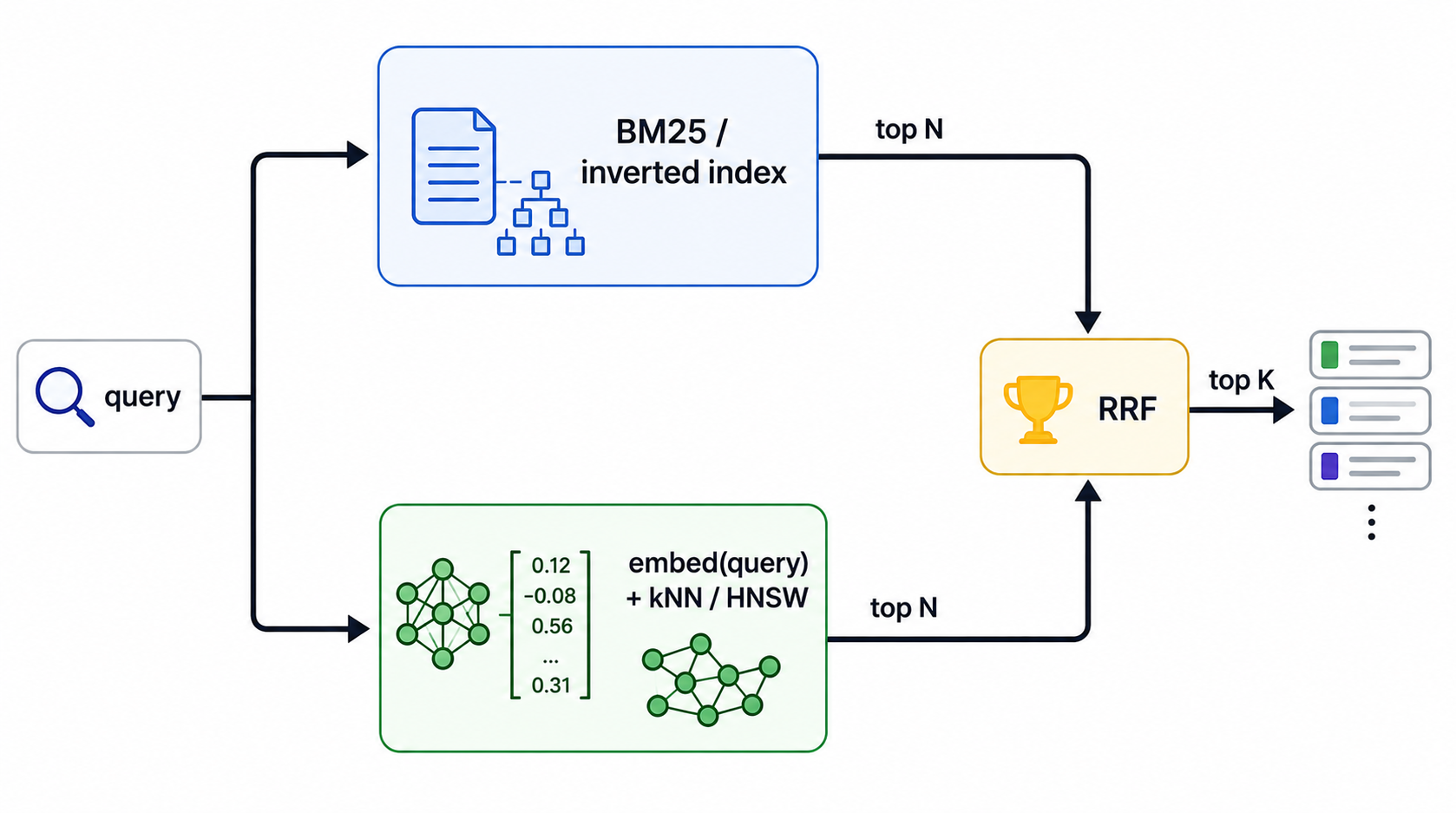
Three things here change your results in practice.
Both searches run in parallel, so latency is the max of the two, not the sum. If BM25 takes 12 ms and vector takes 25 ms, the search costs 25 ms plus fusion, and fusion is noise: sorting a few dozen items in memory won’t show up in your p99.
The real bottleneck is usually generating the query embedding. If you’re calling an external API, every search becomes a network round trip before you even touch the index, and that typically dominates total time. Two ways out: cache query embeddings, which works remarkably well because query distribution is heavily concentrated in the short head (the same phrases repeat all day long), or run the model yourself. A small embedding model on CPU already changes that math.
Fusion window size matters more than k. If each side returns only 10 candidates, a document sitting at position 11 in both lists simply doesn’t exist as far as RRF is concerned. Your hybrid recall is capped by the union of the two candidate sets. In Elasticsearch that parameter is rank_window_size and it defaults to 10, which is far too small for almost any real use case. Pulling 50 or 100 per side and truncating afterward is often the difference between “works” and “why doesn’t this obvious result show up?”.
Fifteen lines of Python, or one line of JSON
Writing RRF from scratch is almost embarrassingly simple:
from collections import defaultdict

def rrf(rankings: list[list[str]], k: int = 60) -> list[tuple[str, float]]:
    """Fuses ranked ID lists. Each list arrives sorted from most to least relevant."""
    scores = defaultdict(float)
    for ranking in rankings:
        for position, doc_id in enumerate(ranking, start=1):
            scores[doc_id] += 1 / (k + position)
    return sorted(scores.items(), key=lambda item: item[1], reverse=True)


bm25   = ["C", "A", "B", "E", "D"]
vector = ["D", "A", "E", "C", "B"]

rrf([bm25, vector])
# [('A', 0.032258), ('C', 0.032018), ('D', 0.031778), ('E', 0.031498), ('B', 0.031258)]
Notice the function knows nothing about search. It takes lists of identifiers. That’s a property, not an accident: you can fuse three, four, five rankers, including business rules and popularity ordering, without changing a line.
In practice you probably won’t write it, because the engines ship RRF already:
GET /products/_search
{
  "retriever": {
    "rrf": {
      "retrievers": [
        { "standard": { "query": { "multi_match": {
            "query": "running shoes for hot weather",
            "fields": ["title", "description"]
        }}}},
        { "knn": {
            "field": "embedding",
            "query_vector": [0.21, -0.05, "..."],
            "k": 50,
            "num_candidates": 200
        }}
      ],
      "rank_constant": 60,
      "rank_window_size": 100
    }
  },
  "size": 20
}
In Elasticsearch, rank_constant already defaults to 60 and rank_window_size defaults to 10, so both fields above are spelled out on purpose. One planning detail that catches teams off guard: RRF in Elasticsearch is a paid feature, listed by Elastic itself among Platinum and Enterprise capabilities. On a self-hosted cluster with a Basic license, the query comes back with a license error.
OpenSearch added rank-based fusion in 2.19 through the score-ranker-processor with the rrf technique, also defaulting to a rank constant of 60, and it’s open source. Qdrant exposes Fusion.RRF directly in the Query API. Weaviate offers rankedFusion, which is RRF, and relativeScoreFusion, which is score normalization, with the latter as the default since 1.24. If you’re on Postgres with pgvector there’s nothing native: it’s two CTEs with row_number() and a full outer join, which works fine too.
Where hybrid wins with no effort at all
Two query patterns show up in basically every domain.
Intent descriptions, in e-commerce. Someone types “dress for a beach wedding”. BM25 chases “dress”, “beach” and “wedding” and brings back a heavy formal gown, a beach cover-up, and maybe a flower girl dress. Vector search understands the context (light, flowing, breathable fabric, long cut, outdoor formal event) and returns the right category, then falls apart the moment the shopper adds “Zara” or a specific model number. Fused, vector search defines the right candidate set and BM25 keeps the literal term anchoring the top.
Technical support and FAQs. Someone searches “401 error”. One article in your knowledge base explains that authentication fails when the token expires, talks about Bearer, JWT and refresh tokens, and never writes the number 401 anywhere. Vector search finds it. At the same time you have a troubleshooting doc with HTTP 401 literally in the first line, and that’s probably the one the user wants first. Vector alone buries the second, BM25 alone never finds the first. RRF puts both on page one.
What both cases have in common is exactly what makes hybrid good: the errors are independent. When one ranker fails, the other fails differently.
Where RRF breaks
This is where I part ways with the internet’s default enthusiasm for the technique.
RRF is blind to magnitude, and that cuts both ways. Ignoring scores is precisely what solves the scale problem, and it’s also what prevents the algorithm from knowing the entire vector list is garbage. If the best similarity in that list was 0.31, RRF still grants it full voting power, because all it sees is “first place”. Score-based methods like Weaviate’s relativeScoreFusion or Qdrant’s DBSF exist for exactly this reason. If one of your retrievers frequently has nothing good to offer in your domain, measure both approaches.
The output scores mean nothing. Look at the table: 0.032258 against 0.031258. Every result lives squeezed into a tiny band, and the value isn’t comparable across queries. That kills anything that depends on a threshold. You can’t say “only show results above X”, and you can’t say “if the score is low, render the empty state”. If your product needs that decision, you’ll need a different signal, usually a raw ranker score captured before fusion.
A wrong document with consensus stays on top. That’s the dry-fit tee holding second place. RRF orders, it doesn’t judge relevance.
Exact identifiers get diluted. If the user types SKU-A4729, the desired behavior isn’t fusion, it’s exact match dominating everything. Hybrid can push up a mediocre document that shows up decently in both lists. The fix isn’t tuning k, it’s detecting the query pattern and routing around the hybrid pipeline before it starts.
If both rankers agree too much, you’re paying for two searches and getting one. Fusion only adds value when the lists disagree. Measure the overlap between the two top 20s on real traffic. If it’s very high, vector search is probably just reproducing BM25, and the problem is your embedding model or what you chose to index.
The operational cost is real. Two indexes over the same corpus, two write paths that need to stay consistent, and one detail that’s easy to forget: filters (category, stock, permissions) have to be applied on both sides, with identical criteria, before fusion. Filtering after fusion wrecks pagination and result counts. Switching embedding models means reindexing everything, and while the reindex runs you have two generations of vectors in the same index.
How to start, and what to measure
The sequence that avoids rework:
- Turn on hybrid with equal weights and
k = 60. Don’t touch anything else yet. - Build a small, honest evaluation set. Somewhere between 50 and 200 real queries from your logs, with relevant documents labeled by hand. It’s half a day of tedious work and it’s the only way to know whether any later change helped.
- Measure three things against baselines: nDCG@10, Recall@50 and MRR. Compare hybrid against BM25 alone and against vectors alone.
- If hybrid doesn’t beat both, stop and investigate. It’s usually a fusion window that’s too small, an embedding model that doesn’t fit your vocabulary, or the wrong field indexed. It isn’t
k. - Only after that should you touch
rank_window_size, then per-ranker weights, andklast.
The order matters. Weights and k are the most visible knobs and the ones that pay off least.
There are libraries for the evaluation side, like ranx, which implements RRF alongside other fusion methods and all the standard metrics. Using it for offline comparison is faster than writing your own nDCG.
The last 10%
Hybrid search with RRF is, in my opinion, the best return on effort in search today. You switch it on, you calibrate nothing, and the result is consistently better than either side alone. For most products, this is where you can stop.
But look at the limit that surfaced along the way: RRF orders by positional consensus, and consensus isn’t the same thing as relevance. The t-shirt stayed in second place because both searches found it plausible, and neither ranker ever read the query and the document together to decide whether one answered the other.
That’s what a cross-encoder does. It takes the 50 or 100 candidates hybrid retrieved, processes query and document in the same forward pass, and reorders them with an understanding no first-stage retriever can have. It’s far too expensive to run over the full catalog, which is exactly why it only makes sense on top of good retrieval.
When you want a perfect top 10 rather than a decent top 100, that’s the next step. Saving it for the third post.
Before then, if you already have BM25 and vector search running separately, today’s experiment is short: grab twenty real queries, save both rankings, fuse them with the fifteen lines of Python above, and eyeball what changed in the top 5. You’ll know in an afternoon whether your domain needs this, and you’ll probably find out where each of your two searches is failing badly.
References
- Cormack, G. V., Clarke, C. L. A., Büttcher, S. Reciprocal Rank Fusion outperforms Condorcet and individual Rank Learning Methods. SIGIR 2009. PDF
- Elasticsearch docs: RRF retriever and reciprocal rank fusion
- Elastic, Pricing FAQ, on RRF availability per subscription tier
- OpenSearch, score-ranker-processor and the 2.19 RRF announcement
- Qdrant, Hybrid Queries
- ranx, a fusion and ranking evaluation library
Second post in a series on modern search. The first one is Semantic Search. The next closes it out with cross-encoder reranking. If you’re building hybrid search somewhere, tell me how it’s going.
› Continue reading

Reranking with Cross-Encoders: the step that separates good search from excellent search
Hybrid search ranks by consensus, and consensus isn't relevance. A cross-encoder reads the query and the document together and reorders your top 100. Third and final post in the series on modern search.

Semantic Search: teaching machines to understand intent, not just words
BM25 still works, but it has four serious blind spots. Embeddings turn text into geometry — and that's the foundation of everything that's hyped in AI today. First in a series on modern search.
Comments
No signup needed. Basic markdown supported. Validated with Cloudflare Turnstile.